Chaos
*Download or directly view image files for higher resolution.*
Jump to section:
Logistic Map
The logistic map is defined by \( x_{n+1} = f_r({x_n})\) with \( f_r(x) = r x (1-x) \), with \( 0 \leq x \leq 1 \) and \( 0 \leq r \leq 4 \).
These images were generated with logistic.py.
Bifurcation Diagrams
Bifurcation diagrams show steady-state orbits at different \(r\) values. These plot \(x\) vs. \(r\) (with parameter \(r\) on the horizontal axis). Several initial data are chosen randomly at each \(r\) value and propogated for thousands of steps. Only the final several hundred steps are plotted at each \(r\) value to isolate steady state behavior. Number of attractors doubles repeatedly as chaos is approached.


Cobweb Diagrams
Cobweb diagrams provide a simple way to visualize time evolution of the map. They can be produced easily by hand by repeatedly reflecting along the x=y diagonal (blue), then tracing back to the plot of \(f(x)\) (black). The horizontal axis is \(x\). You can observe different types of and numbers of attractors at various parameter values.


Chirikov Map
Images below are for the Chirikov map \[ p_{n+1} = p_{n} - K \sin(x_{n}) \] \[ x_{n+1} = x_{n} + p_{n+1} \] with \( -\pi \leq x < \pi \) and \( -\infty < p < \infty \).
These images were generated with chirikov.py.
Poincare Plot
The approach to chaos is evident as certain orbits become space-filling.

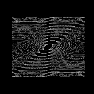
Chaotic Art
Some fun images generated by adding randomness to bifurcation diagrams and Poincare plots.